MLE Using R and an Endangered Species Example
What is difference between OLS and MLE?
OLS and MLE both estimate a model made up of parameter estimates that describes the relationship between two or more variables. Most of time we are interested in a point estimates, or the mean impacts of some random variable X on outcome Y in the population, and the uncertainty around its mean (often referred to as Greek betas, sigma, etc.). A fundamental problem for all model estimates and methods of deriving them is that the population cannot be fully observed in most cases. If it were, statistical methods would not be needed. Estimates, regardless of how they were derived, instead approximate relationships in the population using samples.
The three primary estimation techniques above could also be technically applied to an infinite different number model types. Selecting a model and its estimation procedure should be based on the question we are asking, the observations available, and most important the the process that we think generated them (linear, binomial, poison, mixed etc.), along with some more formal comparisons of fit and explanatory power which I’ll discuss below in 1b.
OLS Description
- Ordinary least squares (OLS) estimates using a fixed set of linear perimeters that minimizes the sum of squared residuals, where residuals are made up of the difference between the fitted “regression” line and the observed data points, Y. The outcome of this OLS fitting process for 1 variable is 3 parameters–alpha, beta, and and error term. That is, an intercept, a slope, and an error that represents all other factors effecting Y, but not observed.
MLE Description
-
Maximum likelihood arrives on beta and other parameters from a different procedure than OLS. Instead of minimizing errors between data and a presumably linear function of (x), ML asks what is the value of the parameter(s) that most likely produced the data. It does not implicitly say anything about errors, but instead forces us to define some probability function that characterizes the data.
-
a.) In the most simple case we might just ask what the mean and standard deviation maximizes the likelihood of observing normally distributed data: argmax = P(Y|mu,sigma). The ML solution is the mean and sD that maximizes the product of the individual likelihood of each observation falling within that particular distribution. The mean and standard deviation that best characterizes the observed data, will have the highest ML out of any other alternative.
-
Computationally, there area few different ways to arrive at the ML, but it is typically done through iteration. First you (the computer) picks a mean and fixed SD, and places it somewhere along the data range. You (it) calculates the product of the likelihood that each observation falls under that particular distribution in its particular position. The distribution is then shifted by on unit the products are calculated again. This process repeats until the highest value is found, Which becomes the maximum likelihood estimator of mean. The process fixes the mean, and Iterates again for the SD.
- b.) We can extend the example above by instead asking what is the conditional mean of Y given some vector, x, that maps onto Y through the linear function alpha+beta*X where alpha and beta (and standard deviation sigma), are not parameters to estimate in the likelihood function
\(argmax = P(Y|alpha,beta,sigma)\).
- b.) We can extend the example above by instead asking what is the conditional mean of Y given some vector, x, that maps onto Y through the linear function alpha+beta*X where alpha and beta (and standard deviation sigma), are not parameters to estimate in the likelihood function
-
Maximizing the log of the likelihood function produces consistent solutions to a non-loged model, but can be computationally easier by allowing us to sum individual likelihoods and produces larger values to maximize across. It is also not always needed to search the entire space before finding a maximum. Clever search functions, for example the Newton-Raphson method, observes the rate of change in likelihood as the function moves from possible parameter value to parameter value. Large positive changes warrant a larger move in that direction where smaller changes mean smaller moves. A negative change warrants moving back the other direction on the scale. These this processes repeats until the model “converges”, or there are no more moves left to be made, which is the maximum. Searing for a mean or univariate case, convergence isn’t really a concern, but solving for many parameters can be multi peaked, require more sophisticated search functions, and take a good deal of time.
-
The resulting ML estimators in the example a. above should be approximately the same as the OLS model with only an intercept, and the ML solutions for alpha, beta, and sigma, will be approximately the same to a linear model estimated using ols (as long as errors are in fact normal).
-
Example
Consider your hired by a regulatory agency to studying the effects of local commercial fishing activity on fish stocks and endangered species impacts. We are concerned with the effects of fishing effort (# of sets) on three outcomes–the number of fish (lets say tuna) caught by the fleet, whether or not they caught an endangered species, and specifically how many endangered turtles were caught. For this we are given a sample of daily data on the number of nets set by the fleet, and corresponding numbers of tuna caught, an indicator of whether an endangered species was caught, and how many of those were turtles. We assume that activity is fully observed, and measured correctly.
The sample is as follows:
#Since I don't have real data, I'll simulate some to fit the problem example
set.seed(2757) #make reproducible
sets<- rnorm(1000,30,10) #Generate 20 normally distributed set numbers
sets<-round(sets) #cant make a fraction of sets so...
fish<- 3*sets+rnorm(1000,0,20) #make outcome roughly 3 times the size of sets (just because you can usually catch >1 fish in a net) with random noise added, also drawn from a normal.
fish<-round(fish)

fishdata<-data.frame(fish,sets)#combine into a dataframe
plot(sets,fish)
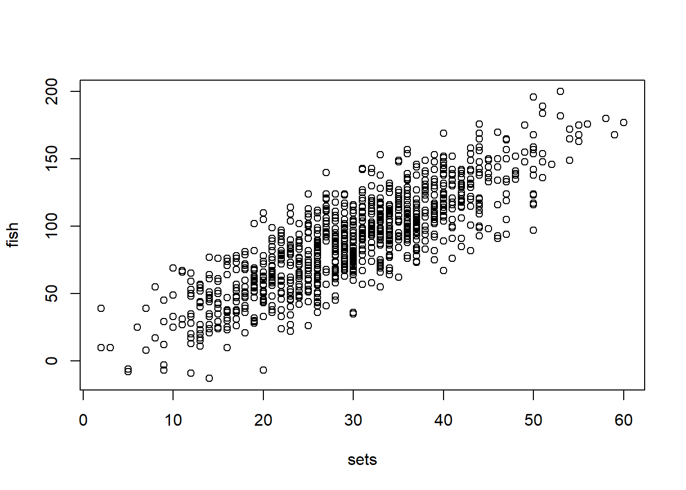
There is a clear relationship between the number of sets made and fish caught (because we made it that way, but still). Now we want to estimate what that actual relationship is, or the effect of x- sets, on Y fish caught. The relationship appears linear, and continuous, so we can propose a linear model which I estimate below using OLS and MLE:
OLS Example
I’ll show this in as much detail as possible using scalar algebra:
OLSestimators<-lm(fish~sets)
summary(OLSestimators)
##
## Call:
## lm(formula = fish ~ sets)
##
## Residuals:
##     Min      1Q  Median      3Q     Max
## -67.481 -13.172  -0.229  12.933  58.666
##
## Coefficients:
##             Estimate Std. Error t value Pr(>|t|)
## (Intercept)  0.89936    1.97770   0.455    0.649
## sets         2.97907    0.06267  47.533   <2e-16 ***
## ---
## Signif. codes:  0 '***' 0.001 '**' 0.01 '*' 0.05 '.' 0.1 ' ' 1
##
## Residual standard error: 19.58 on 998 degrees of freedom
## Multiple R-squared:  0.6936,	Adjusted R-squared:  0.6933
## F-statistic:  2259 on 1 and 998 DF,  p-value: < 2.2e-16
MLE Example
Performing a MLE by explicitly defining parameters for the linear model:
require(stats4)
## Loading required package: stats4
y<-fish
x<-sets

LogLiklihood<-function(alpha,beta,sigma) { #this does the work of summing individual likelihoods given our set parameters, model, and distribution

Likelihood= dnorm((y-alpha - beta *x),0,sigma) # define parameters alpha, beta,and sigma and return the likelihood of x

-sum(log(Likelihood)) #sums the log of the likelihoods of each individual from above
}
Technically, we could start plugging in a bunch of guesses into our function until we find the combination that give us the highest likelihood of producing Y. The function and and optimization algorithm we run after this minimizes a negative likelihood, so in this case the smaller number corresponds to a higher liklihood #e.g. the log liklihood of intercept=1, beta=5, and sigma 10 is:
LogLiklihood(1,5,10)
## [1] 25530.29
And the log likelihood when intercept=1, beta=5, and sigma 10 is:
LogLiklihood(2,6,15)
## [1] 25117.12
Clearly the parameter values that produced the smaller (negative) likelihood is the more likely values that produced the data, but we can do better by running an optimization algorithm as described above to find the maximum:
MaxLike<- mle(LogLiklihood, start = list(alpha=1, beta=5, sigma=10)) #This iterates over the log likelihoods until the maximum is found. Here we set some starting values that we think might be close to the actual values so that the search algorithm can search more efficiently.

summary(MaxLike) #Report the value alpha, beta, and sigma that maximized the probability of observing the data, y
## Maximum likelihood estimation
##
## Call:
## mle(minuslogl = LogLiklihood, start = list(alpha = 1, beta = 5,
##     sigma = 10))
##
## Coefficients:
##        Estimate Std. Error
## alpha  0.899206 1.97571678
## beta   2.979065 0.06261043
## sigma 19.562329 0.43742656
##
## -2 log L: 8785.09
When might you use MLE?
Note that the parameters found by OLS and ML approximately found the same values even though they are fundamentally different techniques. This is because the the assumption of the OLS model were written directly into the ML function. In this way the technique you use is irrelevant. The better question is whether the assumptions hold that make OLS or it’s ML counterpart the best linear unbiased estimator (“BLUE”) of the population its drawn from. That is:
- Linear Parameters
- This simply means that the model is linear in its parameters. That is the alpha, and beta values do not change. Variable input, x, can vary. Including higher order terms, like polynomials, does not violate this assumption, nor does transforming variables befor estimation. For example, when regressing log(Y) on X the beta associated with that relationship is still fixed and linear. The parameters become non-linear and violate this condition if the effect of x on y varies depending on the value of x (e.g. logit).
Practically some books categorize this simply as “the linear model describes the data”, or is the appropriate model. If not, the assumption is violated.
- Errors are uncorrelated/independence/no endogeneity
- This is a key assumption, but one that is difficult to prove and takes up a good deal of our time trying to convincingly show. For our estimators to be unbiased, unexplained variation must be random (stochastic).
From a practical standpoint we are assuming that treatment in our sample is as good as randomly assigned, after conditioning on observable traits that might affect treatment and outcome–hence the term “the effects of X1 on y after controlling for/conditioning on x2…xn”, or after controlling for the probability of selection into treatment brought on by xn. This can take on a few different forms. Most obvious (to me) is when a variable is left out of the model that effects both x and y, knows as omitted variable bias, the direction of which depends on the +/- relationship between x and y and x and the omitted var. Other forms of the problem include autocorrilation between a variable and itself across time and space, and simultaneity which occurs when levels of x are determined bY the outcome, which is often the focus of spatial and temporal lagged variables, and instruments (to identify independent variation).
- The expected value of the error term is zero
- Just means that the fitting process was sucsesfull
- Homoskedacticity
- equall error variance across levels of X important for inference
- No perfect coliniarity
- <1 is ok, but if perfect there is no solution
Its nearly impossible to satisfy these assumptions exactly, but we could conclude they fit our example reasonably well. The assumption most likely violated is uncorrelated errors. The number of sets made is likely corrilated with the size and technology of a fishing vessel, as well as the expertise of the fishermen. If higher set days are positively correlated with some other technical advantage, and that technical advantage leads to higher catch the coefficent on sets will be biased upward, when its really technical knowledge driving fishing outcomes. Importantly, this would be an identification issue with any model type (without collecting more/different data), so OLS is still appropriate.
When OLS is not best
But what about when the data generating process is non-continuous, errors are not normal etc. such that conditions become violated. In this case a linear model is not likely to be the best fit to the data, and is certainly not un-biased.
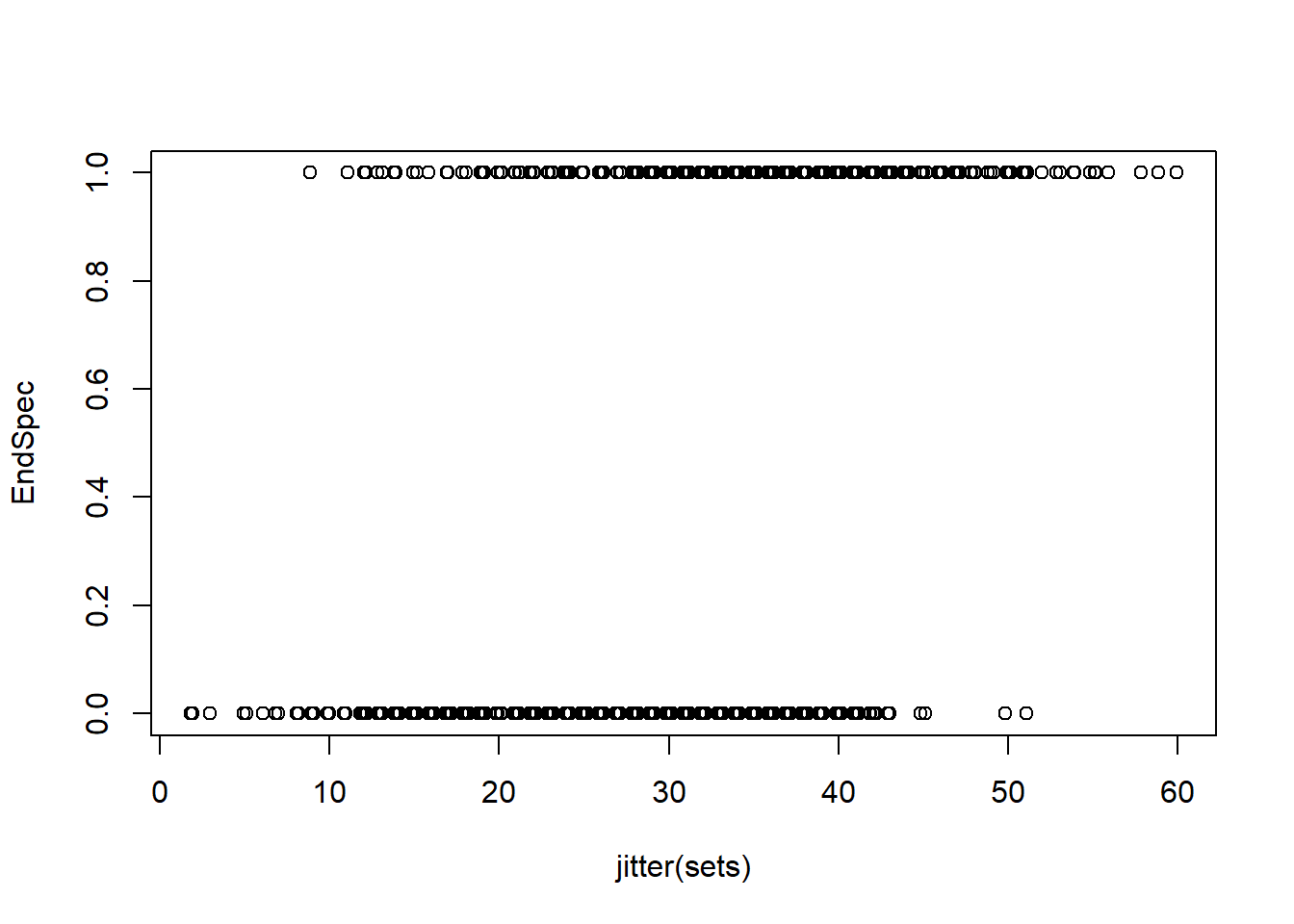
Consider the same example above, expect the agency next asks you to estimate the impacts of sets on endangered species impacts. Now we are concerned with the effects of fishing effort (# of sets) on whether or not they caught an endangered species, and additionally how many endangered turtles were caught. As before we are given a sample of daily data on the number of nets set by the fleet, and an indicator of whether an endangered species was caught, and how many of those were turtles. We again assume that activity is fully observed, and measured correctly.
set.seed(42)
EndSpec<- ifelse(sets > mean(sets)+rnorm(20,0,10),1,0) #make a dichotomous variable representing endanger species takes
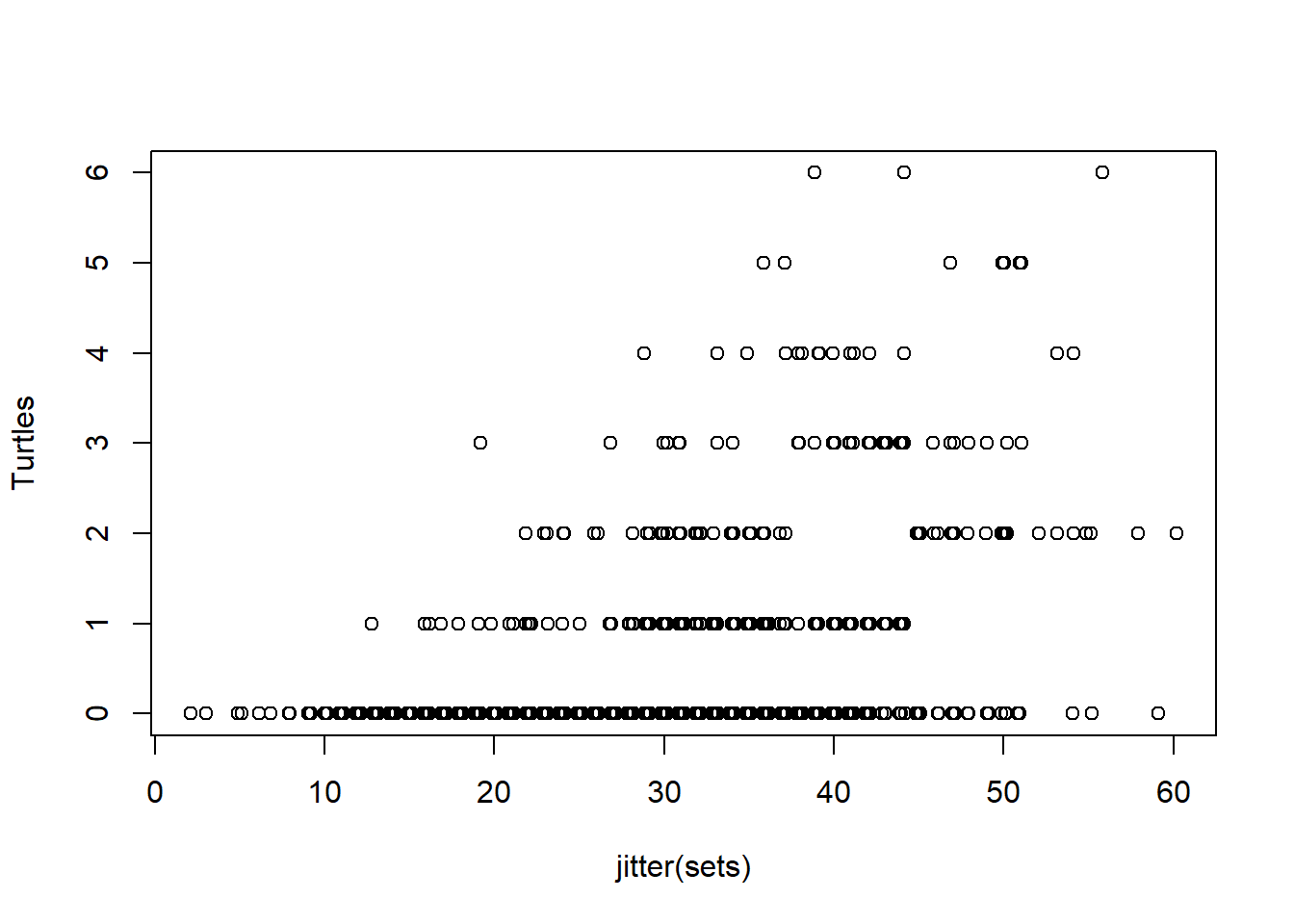
Turtles<-round(ifelse(EndSpec>0, rpois(1000,lambda=1)*sets/30,0)) #make a count variable as a function of sets when EndSec>0 and some random error
plot(jitter(sets),EndSpec)
plot(jitter(sets),Turtles)
hist(Turtles)
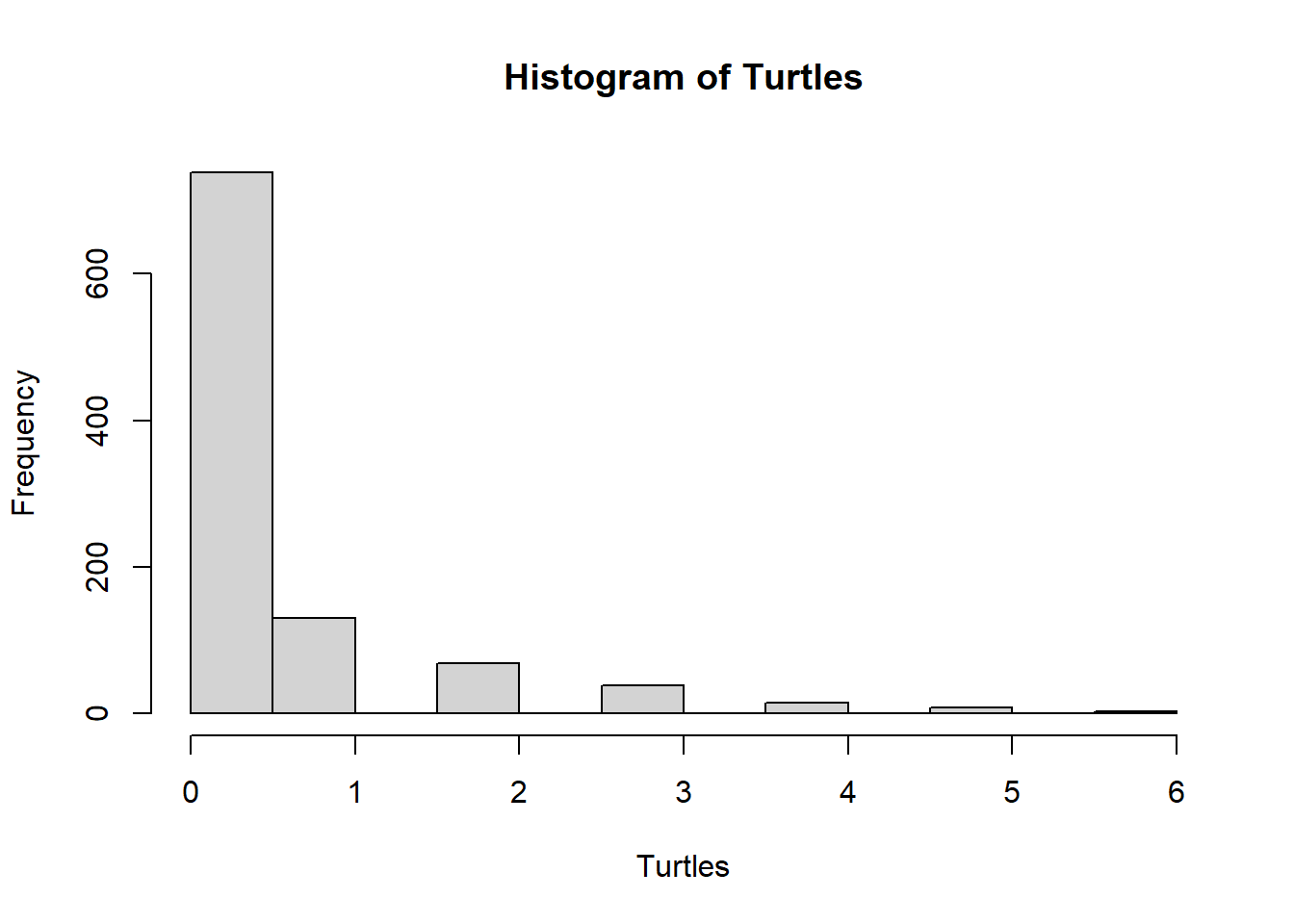
table(Turtles)
## Turtles
##   0   1   2   3   4   5   6
## 738 130  68  38  15   8   3
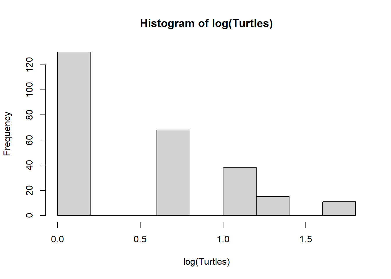
hist(log(Turtles))
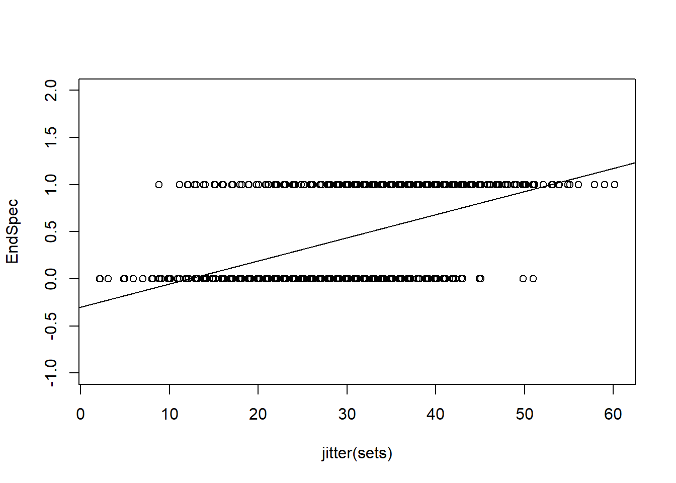
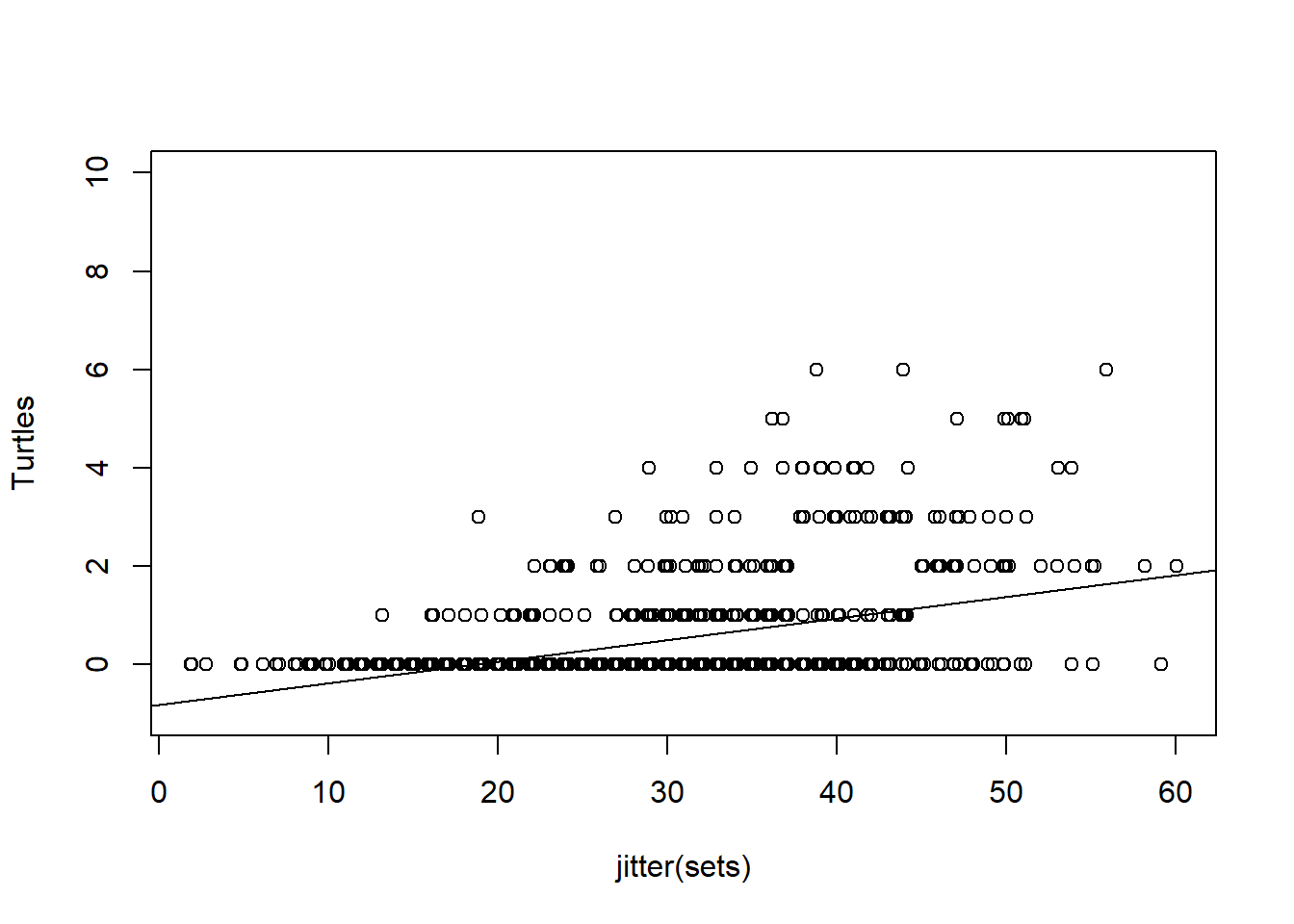
We could consider linear models, but its quickly obvious a linear model will estimate nonsense values
EndSpecLine<-lm(EndSpec~sets)
plot(jitter(sets),EndSpec, ylim=c(-1,2))
abline(lm(EndSpecLine))
TurtleLine<-lm(Turtles~sets)
plot(jitter(sets),Turtles, ylim=c(-1,10))
abline(lm(Turtles~sets))
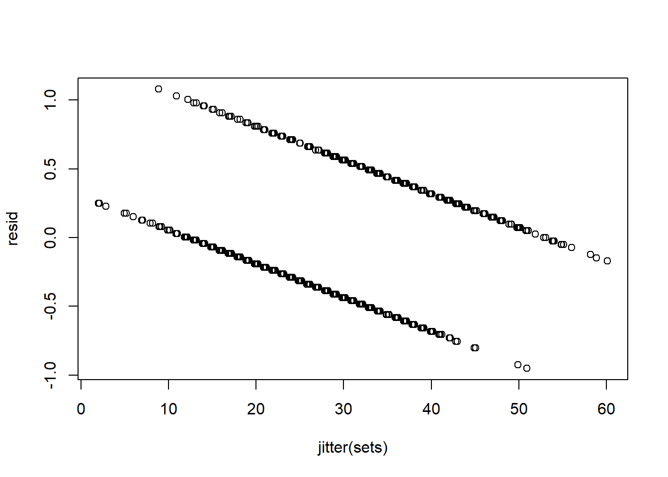
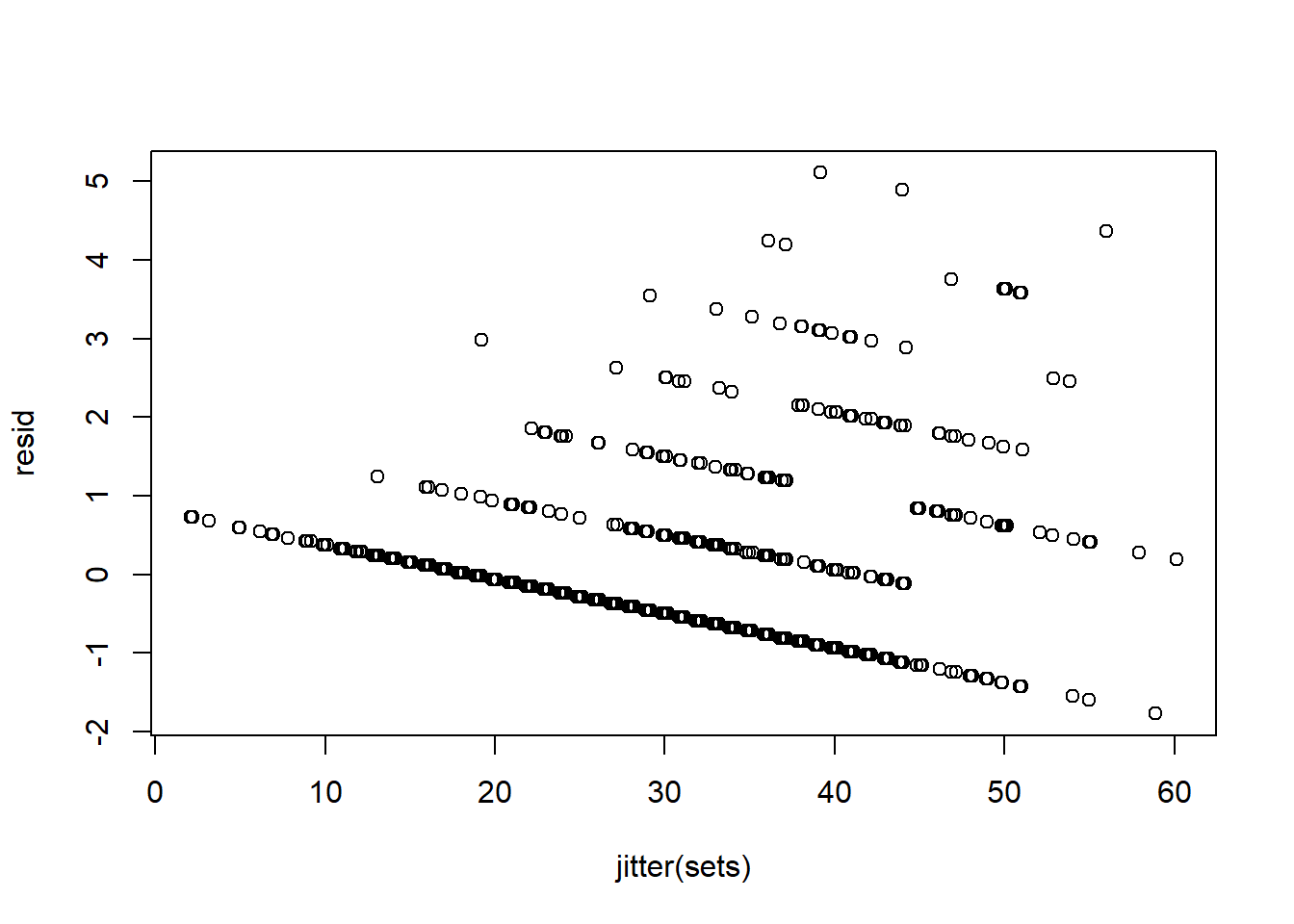
And that residuals are not normal, zero mean, homoskedastic etc..
resid<-residuals(EndSpecLine)
plot(jitter(sets), resid)
resid<-residuals(TurtleLine)
plot(jitter(sets), resid)
Models for non-continuous dependent variables
Once we determine that OLS is not the BLUE, and risks giving nonsensical predictions, we can look to other models that map x onto y in a way that is more consistent with the generating process. The following fit alternative models.
Any Endangered species (Binary Dependent Var)
Instead of estimating a linear model through points about 0 and 1, the Probit model allows us to fit a function to the log odds of y: \(log(P(y=1| x)/P(y=0|x))\) , the log of the probability that y=1 divided by the probability y is 0. The new scale of y is said to be the “latent”, or unobserved variation in Y and is now continuous between -infinity & infinity. Another useful property is that when the odds of y given x is 0.5 (e.g a toss of a fair coin), the log odds =0 such that any value above 0.5 is positive and any value lower than 0.5 is negative. That is, instead of the effects of X on Y directly, I am now concerned with whether X affects the odds of observing y beyond an unconditional coin toss, and by how much.
y<-EndSpec
x<-sets

LogLiklihoodLogit<-function(alpha,beta) { #this does the work of summing individual likelihoods given our set parameters, model, and distribution

likelihood = y*plogis(alpha+beta*x)+(1-y)*(1-plogis(alpha+beta*x)) # first define parameters alpha and beta in a binomial process P(1,0|x), then wrap that inside a logit link (could use a probit/pnorm link etc.) to define how x maps onto y.

-sum(log(likelihood )) #sums the log of the likelihoods of each individual from above
}

MaxLike<- mle(LogLiklihoodLogit, start = list(alpha=-4, beta=.1))
summary(MaxLike)
## Maximum likelihood estimation
##
## Call:
## mle(minuslogl = LogLiklihoodLogit, start = list(alpha = -4, beta = 0.1))
##
## Coefficients:
##         Estimate  Std. Error
## alpha -4.2697338 0.306867529
## beta   0.1309167 0.009588519
##
## -2 log L: 1097.769
logitfit<-glm(y~x, family=binomial(link="logit"))#Check my LL function using a canned version
summary(logitfit) # approximately the same
##
## Call:
## glm(formula = y ~ x, family = binomial(link = "logit"))
##
## Deviance Residuals:
##     Min       1Q   Median       3Q      Max
## -2.2326  -0.8853  -0.4361   0.9453   2.5038
##
## Coefficients:
##              Estimate Std. Error z value Pr(>|z|)
## (Intercept) -4.267600   0.306788  -13.91   <2e-16 ***
## x            0.130853   0.009586   13.65   <2e-16 ***
## ---
## Signif. codes:  0 '***' 0.001 '**' 0.01 '*' 0.05 '.' 0.1 ' ' 1
##
## (Dispersion parameter for binomial family taken to be 1)
##
##     Null deviance: 1369.3  on 999  degrees of freedom
## Residual deviance: 1097.8  on 998  degrees of freedom
## AIC: 1101.8
##
## Number of Fisher Scoring iterations: 4
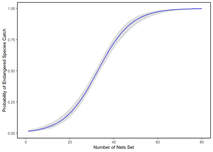
This is technically the conclusion of the binary response/latent variable model…but thinking about changes in log odds is pretty cumbersome. More useful is to report the expected probability of y back on a 0-1 scale, which can be derives by applying an inverse function to the coefficient (distribute back to th RHS of the equation). Plugging in values to the inverse logit gives us the usual “s curve” that describes the predicted probability of y given x.
Importantly, we can no longer generate predictions above 1 or below zero, and the effects of x on y are not linear. That is, the value of beta varies across different intervals of x, and by construction, different levels of other covariates if in the model.
#define a simulation that take 1000 random draws from a normal distribution described by model estimate and variance.
beta.sim<-mvrnorm(1000, coef(logitfit),vcov(logitfit))

# Make x range 0-80
p<-cbind(1,seq(1:80))

#Generate 1000 draws from p -- the model distribution-- at each 80 levels of x
temp<-plogis(beta.sim%*%t(p))

plot<-as.data.frame(cbind
                    (mean=apply(temp, 2, quantile, 0.5),
                    upper=apply(temp, 2, quantile, 0.975),
                    lower=apply(temp, 2, quantile, 0.025),
                    numsets=seq(1:80))
                   )

plotlogitfit<-ggplot(data = plot,
              aes(x=numsets,
                  y=mean,
                  ymin=lower,
                  ymax=upper))+
              geom_line(color="blue",
                  size=1)+
              geom_ribbon(fill="grey",
                  alpha= .5)+
              theme(panel.background=element_rect(fill="white")) +
              theme(plot.background=element_rect(fill="white")) +
              theme(panel.border = element_rect(colour = "black", fill=NA, size=1))+
              scale_y_continuous("Probability of Endangered Species Catch")+
              scale_x_continuous("Number of Nets Set",
                  limits = c(0, 80))

plotlogitfit
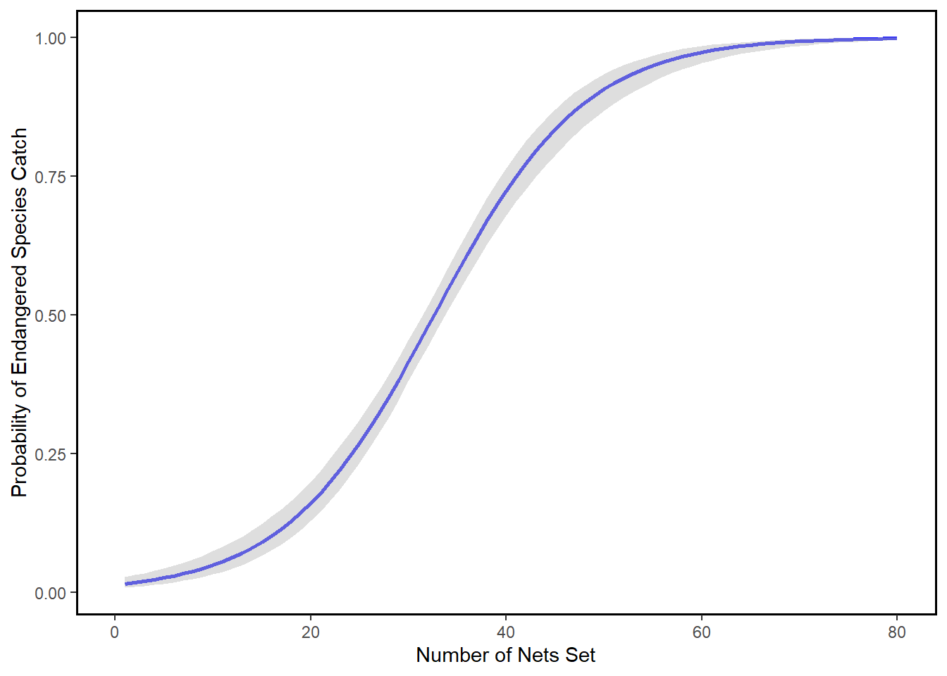
Note again that x number of nets sets by fishermen correspond to some probability of catching an endangered species. For example, when 20 nets were cast:
invlogit<- function(coef) {
  1/(1+exp(-coef))
} #for the sake of completeness, I'll define the inverse logit as a function

 prob20<-invlogit(logitfit$coef[1]+logitfit$coef[2]*20)

 print("the probability of catching an endangered species")
## [1] "the probability of catching an endangered species"
prob20
## (Intercept)
##   0.1610351
We might conclude that this is reasonably low, but we know that 0.16 is not the constant effect of the next 20 sets, so it might not be a good idea to let the fleet add another 20. To be sure, in increase in probability of catching an endangeres species going from 20 to 40 sets is:
prob20to40<-invlogit(logitfit$coef[1]+logitfit$coef[2]*40)-
invlogit(logitfit$coef[1]+logitfit$coef[2]*20)

prob20to40
## (Intercept)
##   0.5633877
Which is a much larger jump, and important more likely than not (>0.5). We can set the log odds to 0, and see that any number of nets allowed above
-logitfit$coef[1]/logitfit$coef[2]
## (Intercept)
##    32.61377
Will give us a probability >.5 and might be a starting point for negotiations in the fishing community.
Count models
The job of the Poisson Regression model is to fit the observed counts y to the regression matrix X via a link-function that expresses the rate vector λ as a function of, 1) the regression coefficients β and 2) the regression matrix X. This link function keeps λ non-negative even when the regressors X or the regression coefficients β have negative values. This is a requirement for count based data.
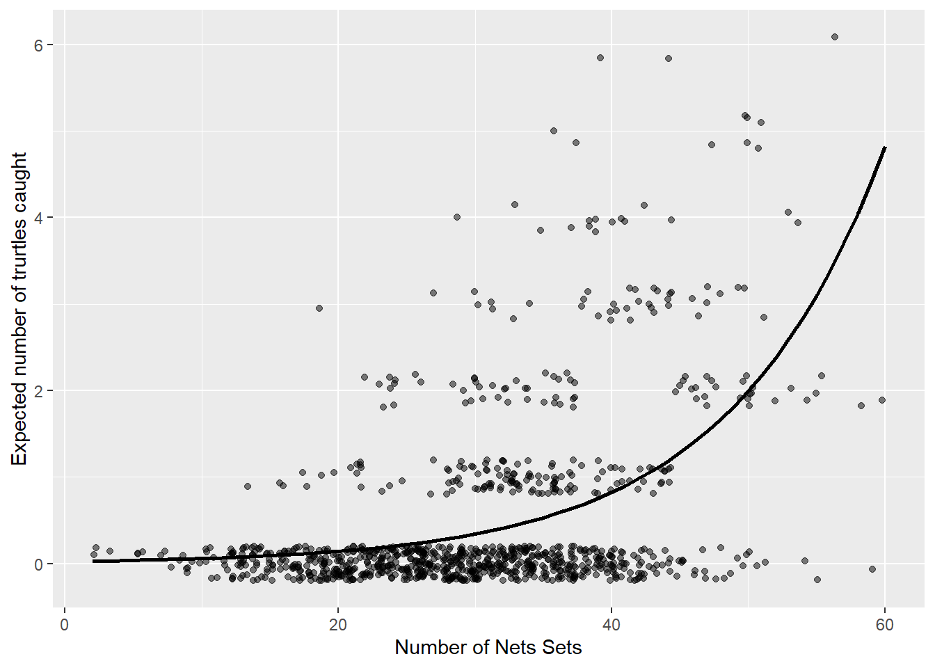
Predicted Turtle Impacts (Count Dependent Var) If we are concerned with zeroing in on turtle counts in particular, the binary response model is not helpful, and the OLS estimator is still bias. Instead we might choose a poisson model whos assumptions about the distribution of y are more consistent with our data. Here we assume that that y >0, can range above 1 and has a variance equal to its mean.
y<-Turtles
x<-sets

LogLiklihoodpoisson<-function(alpha,beta) { #this does the work of summing individual likelihoods given our set parameters, model, and distribution

Likelihood= dpois(y,exp(alpha+beta*x)) # define parameters alpha, beta,and sigma and return the likelihood of x

-sum(log(Likelihood))  #sums the log of the likelihoods of each individual from above
}

MaxLike<- mle(LogLiklihoodpoisson, start = list(alpha=0,beta=0))
summary(MaxLike)
## Maximum likelihood estimation
##
## Call:
## mle(minuslogl = LogLiklihoodpoisson, start = list(alpha = 0,
##     beta = 0))
##
## Coefficients:
##         Estimate  Std. Error
## alpha -3.7181988 0.182918985
## beta   0.0881484 0.004600315
##
## -2 log L: 1756.915
poissonfit<-glm(y~x, family=poisson(link="log"))#Check my LL function using a canned version
summary(poissonfit) # approximately the same
##
## Call:
## glm(formula = y ~ x, family = poisson(link = "log"))
##
## Deviance Residuals:
##     Min       1Q   Median       3Q      Max
## -2.9709  -0.9024  -0.6066  -0.1651   3.7920
##
## Coefficients:
##              Estimate Std. Error z value Pr(>|z|)
## (Intercept) -3.722763   0.183083  -20.33   <2e-16 ***
## x            0.088260   0.004605   19.17   <2e-16 ***
## ---
## Signif. codes:  0 '***' 0.001 '**' 0.01 '*' 0.05 '.' 0.1 ' ' 1
##
## (Dispersion parameter for poisson family taken to be 1)
##
##     Null deviance: 1493.0  on 999  degrees of freedom
## Residual deviance: 1117.7  on 998  degrees of freedom
## AIC: 1760.9
##
## Number of Fisher Scoring iterations: 6
#define a simulation that take 1000 random draws from a normal distribution described by model estimate and variance.
#beta.sim<-rpois(1000, coef(poissonfit))
# Make a design matrix, and x range 0-100
#p<-cbind(seq(1:80))
#Generate 1000 draws from p -- the model distribution-- at each 100 levels of x
#temp<-as.data.frame(ppois(lengthbeta.sim%*%t(p)))
#plot<-as.data.frame(cbind
# (mean=apply(temp),
# numsets=seq(1:80))
# )
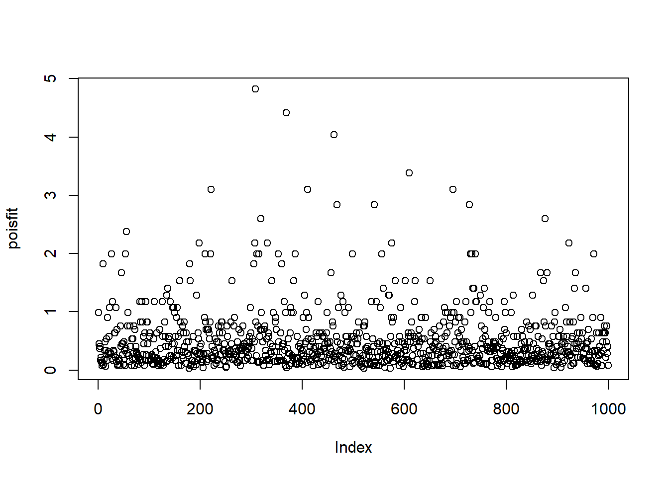
poisfit<-predict(poissonfit, type="response")
plot(poisfit)
data<-as.data.frame(cbind(sets,poisfit, Turtles))

ggplot(data, aes(x = sets, y = poisfit)) +
  geom_point(aes(y= Turtles),alpha=.5, position=position_jitter(h=.2)) +
  geom_line(size = 1) +
  labs(x = "Number of Nets Sets", y = "Expected number of trurtles caught")
visreg(poissonfit,
       scale="response",
       overlay=TRUE)
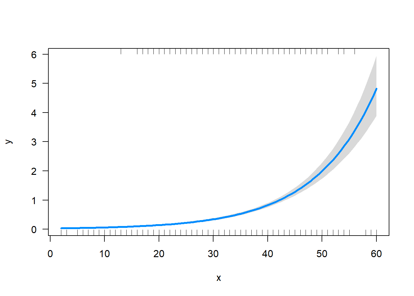
exp(poissonfit$coef[1]+poissonfit$coef[2]*60)
## (Intercept)
##    4.820192